Statistical Analysis
Descriptive Stats Revision
- measures of central tendency:
- describe where most data is clustered, shows the representative characteristic.
- Mean, median, mode.
- measures of spread:
- measuring variability, tells us how much data values differ from the center.
- Range, variance, std.
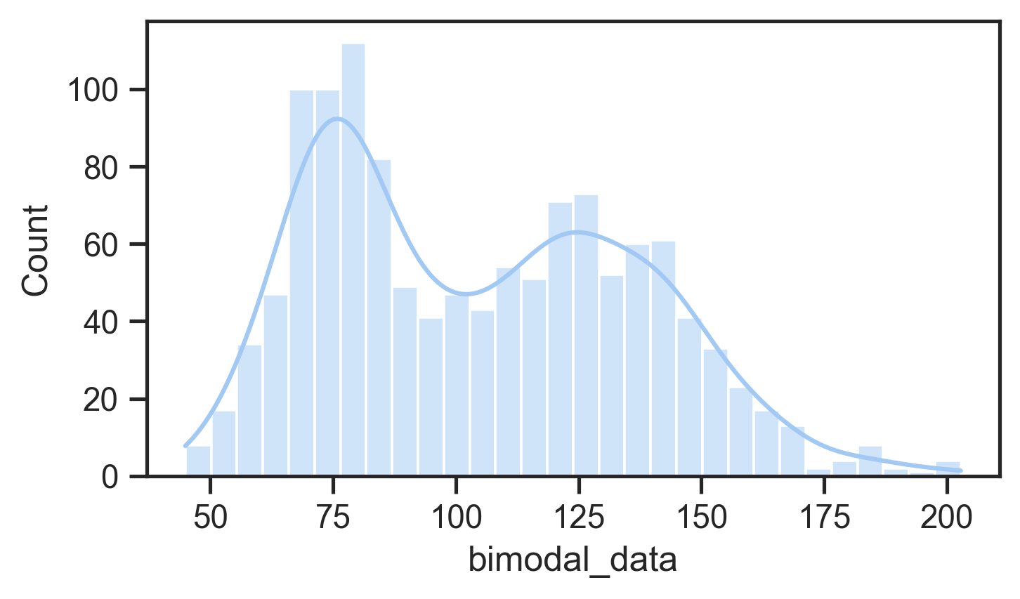
- normal distribution defined by mean and standard deviation
- Many statistical tests (e.g., t-tests, ANOVAs) assume normality
- Can use tests or plots to check for normality
- If not normal: consider data transformation or nonparametric tests

Why compare means
In an evaluation with two groups or conditions, we want to know whether differences are meaningful or not.
- Between-group design: Different participants in each condition.
- Within-group design: Same participants experience all conditions.

Why Not Just Compare Means?
As an example: Is an height difference of 20cm meaningful?
- If talking about adult people, probably yes.
- If talking about mature Eucalyptus trees, probably no.
- Means don’t account for data variance.
So what do we do?
- Significance testing
- Compares explained variance (from independent variable) vs. unexplained variance (random/error).

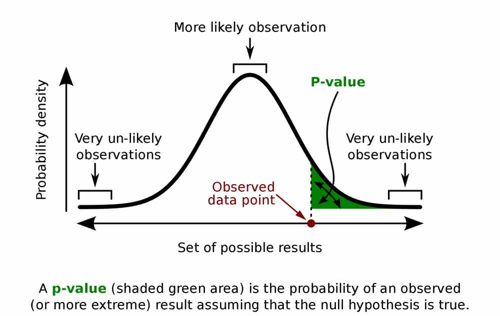
What’s a p-value?
- p-values are thrown around a lot in some scientific fields
- p is the probability of obtaining a measurement by chance given the existing distribution of measurements.
- low p-value = low probability difference occurred by chance: likely a real effect
- low p-value is evidence supporting a hypothesis
A typical cut-off for “significance” is p = 0.05. Is this the best choice?
Analysis of Variance
What if you have more than two groups to compare? (e.g., three+ interface variations?)
What if you have more than one independent variable? (e.g., comparing the individual and combined effects of two separate aspects of an interface)
Analysis of variance (ANOVA) enables these more complicated comparisons.
An ANOVA’s output is a statistic called F so sometimes called an F-test.

Identifying relationships
Understand how variables relate to each other (e.g., is age or experience related to performance?)
Correlation:
- Measures the strength and direction of the linear relationship between two variables.
- Most common method: Pearson’s r: range: -1.00 (negative) to 1.00 (positive). 0 indicates no linear relationship.
Pearson’s r2 (Coefficient of Determination)
- Represents the shared variance between two variables.
- Example: If r = 0.70, then r2 = 0.49, meaning 49% of variance in one variable is explained by the other.
Note: correlation not equal to causation!
Imagine an experiment measuring time spent in an online shopping app vs income.
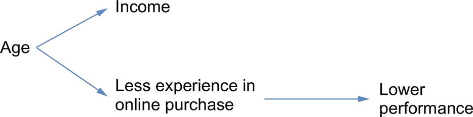
E.g., income vs. performance may be correlated due to an intervening variable (e.g., age) rather than directly related.
Case Studies
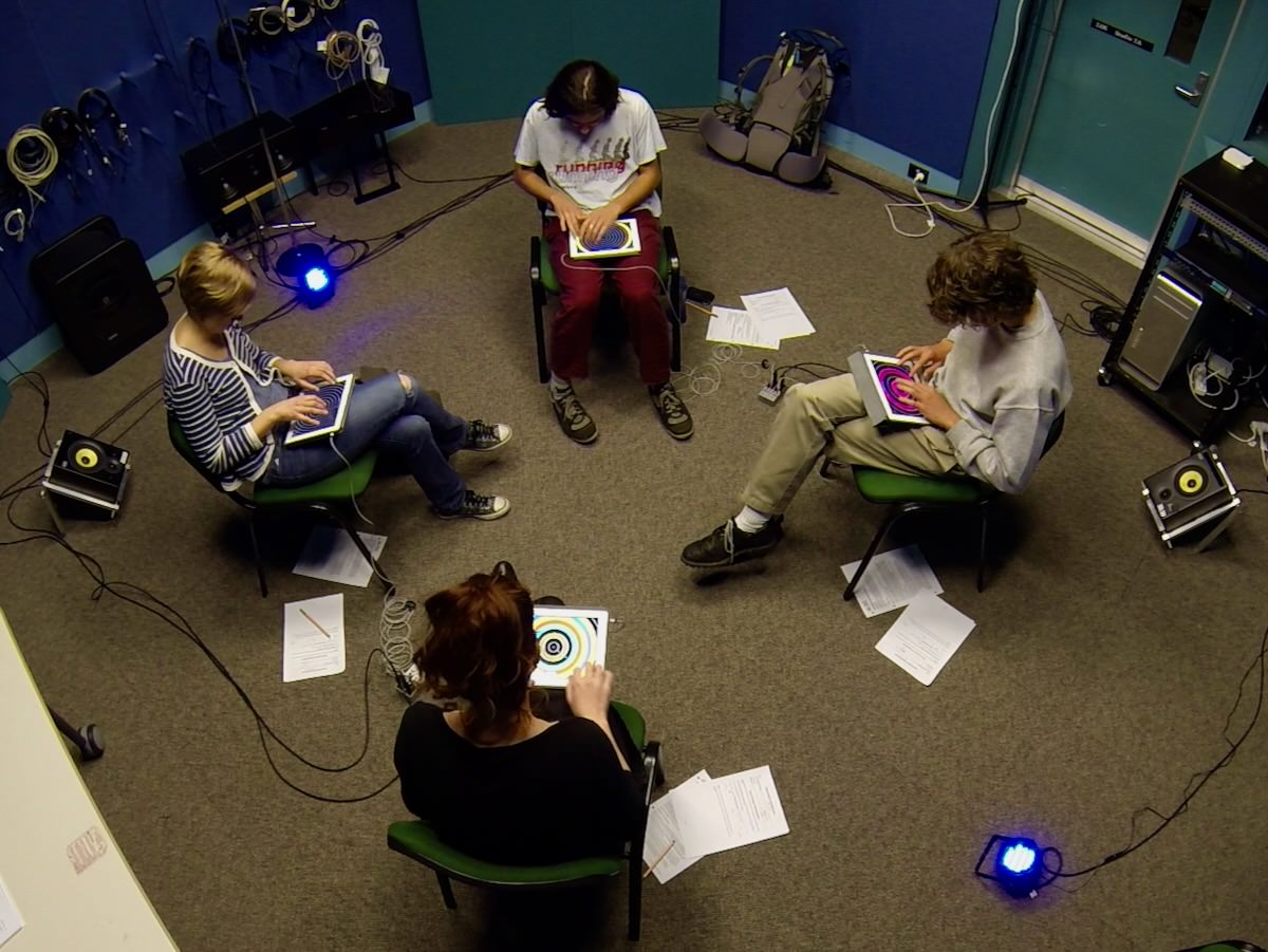
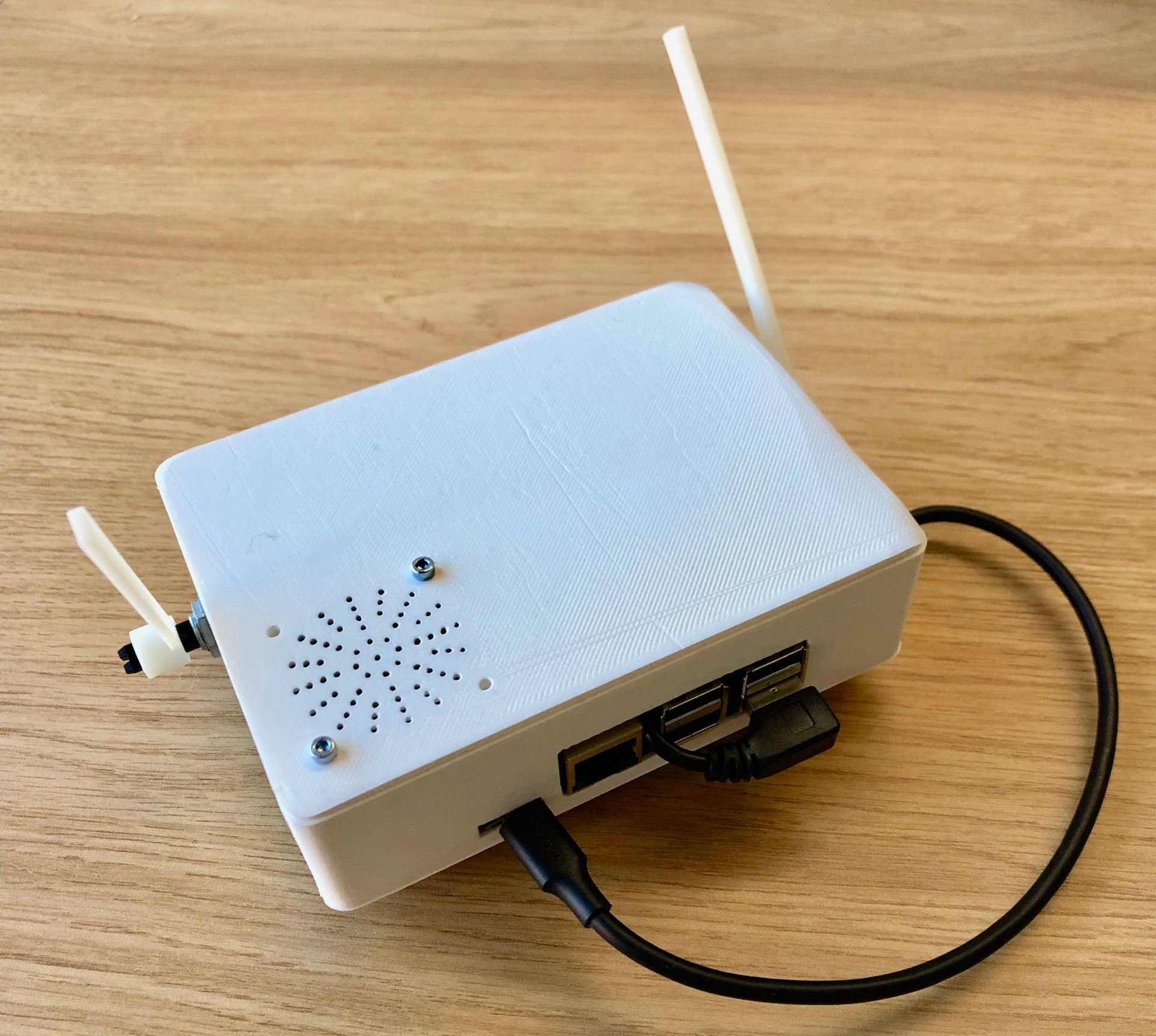
Comparing AI models on a physical musical instrument
Research question:
What effects will different machine learning models and feedback mechanisms have on simple improvised music performances?
“Understanding Musical Predictions with an Embodied Interface for Musical Machine Learning” Martin et al. (2020)
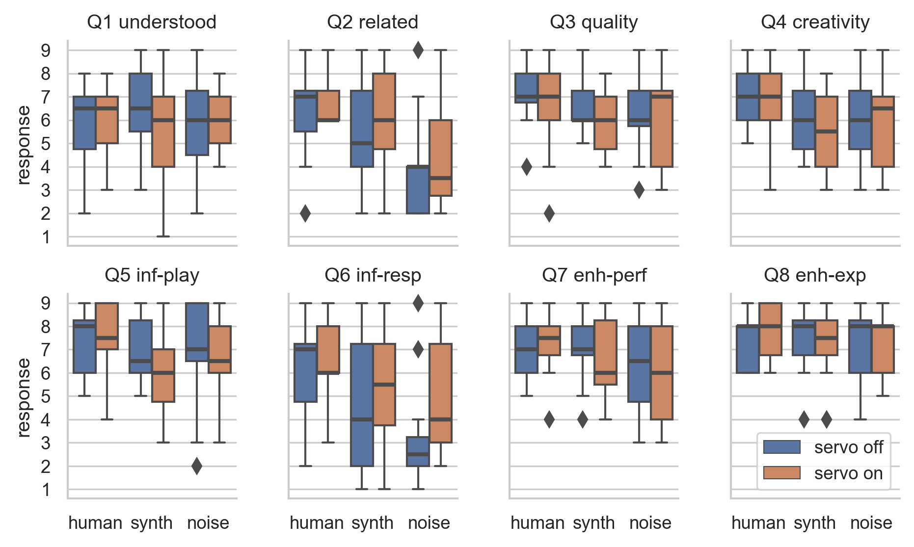
Survey Results: ART ANOVA and pairwise t-tests
- Change of ML model has significant effect: Q2, Q4, Q5, Q6, Q7
- Human model most “related” and “creative”, noise least.
- Noise model not rated badly!
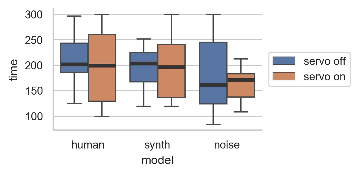
Performance Length
- Human and synth: more range of performance lengths with motor on.
- Noise: more range with motor off.
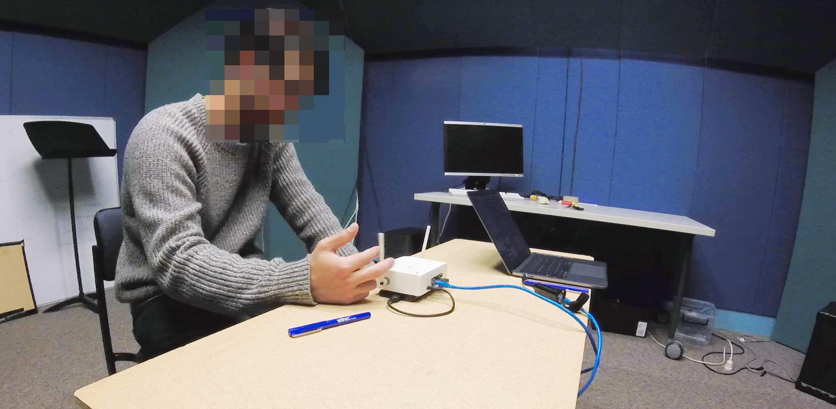
EMPI Takeaways
- Studied self-contained intelligent instrument in genuine performance.
- Physical representation could be polarising.
- Performers work hard to understand and influence ML model.
- Constrained, intelligent instrument can produce a compelling experience.
Questions: Who has a question?
Who has a question?